Motor control overview
FOC current control
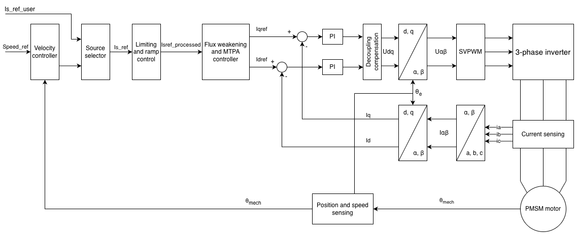
The FOC (Field-Oriented Control) current controller is the innermost and most critical control loop of the inverter. It regulates the d- and q-axis stator currents independently in the rotating reference frame, enabling precise and decoupled control of flux and torque. Its dynamic performance directly determines torque response speed, current waveform quality, and system stability.
The PI current controller gains are computed automatically by the inverter firmware based on the configured motor parameters (L_d, L_q, flux linkage). Correct operation therefore depends on accurate motor parameters. If the parameters are incorrect, the following effects are expected:
| Effect | Description |
|---|---|
| Transient overshoot | Excessive current overshoot during step changes |
| Oscillation / instability | Sustained current oscillation or controller divergence |
| Steady-state error | Incorrect operating point, reduced torque accuracy |
| Increased losses | Higher current ripple, elevated inverter and motor losses |
MTPA and field weakening
MTPA — Maximum Torque Per Ampere
In a permanent magnet synchronous motor (IPMSM) with asymmetric inductance (L_q ≠ L_d), the total electromagnetic torque has two components: the magnetic torque from the permanent magnet flux, and the reluctance torque from the inductance asymmetry. For a given stator current magnitude, the ratio of d- and q-axis currents determines how much of each component is produced.
MTPA continuously calculates the current vector angle that maximizes combined torque output for the instantaneous current demand. The stator current is resolved into the optimal d- and q-axis components while respecting the maximum current circle constraint \(i_d^2 + i_q^2 \leq i_{max}^2\). Compared to operating at zero d-axis current, MTPA reduces copper losses and improves efficiency throughout the base speed region without exceeding the motor's thermal or current limits.
MFW — Magnetic Field Weakening
As motor speed increases, the back-EMF rises proportionally. Once it approaches the available DC bus voltage — the base speed — the inverter can no longer supply sufficient voltage to maintain the full flux current. To operate above the base speed, the inverter injects a controlled negative d-axis current component that opposes the permanent magnet flux and reduces the effective flux linkage. This lowers the back-EMF and allows continued operation at higher speeds within the DC bus voltage limit, at the cost of reduced peak torque capability.
The inverter monitors the magnitude of the output voltage vector and uses it to regulate the d-axis current continuously. Below base speed the output voltage is well within the available limit, so field weakening is not active. As speed rises and the voltage limit is approached, the regulator begins injecting negative d-axis current automatically — no fixed speed threshold or lookup table is required. The q-axis current is adjusted accordingly to keep the operating point within the maximum current circle, ensuring the current limit is respected at all times.
When both MTPA and MFW are enabled, the d-axis current is governed by whichever demand is more negative at any given operating point: MTPA dominates in the base speed region, and field weakening takes over as speed increases beyond base speed. The transition between the two is continuous and requires no operator intervention.
The base speed is determined by the motor flux linkage \(\lambda_{pm}\) and the available DC bus voltage. The inverter calculates when to enter field weakening automatically based on the configured motor parameters.
Enable incrementally
MTPA and MFW must not be enabled until basic motor operation has been verified and encoder calibration is complete. Enable them incrementally as described in the setup procedures.
Fault and limit system
Fault system
When a fault condition is detected, the inverter immediately disables PWM modulation and the motor coasts to a stop. No active braking is applied — the drive simply stops switching and allows the motor to decelerate freely under its own inertia and friction.
The fault remains active for as long as the underlying condition persists. The Fault Stop Time countdown does not begin until the fault condition has cleared. Once the countdown expires without a recurrence, the fault is automatically reset and the inverter resumes executing commands. This mechanism prevents rapid cycling in situations where the root cause has not been resolved.
Each fault is assigned a numeric code that is reported over the CAN bus to assist with remote diagnostics and system integration. The active fault code can also be monitored directly in DTI CAN Tool.
| Code | Name | Description |
|---|---|---|
| 0 | FAULT_CODE_NONE |
No fault |
| 1 | FAULT_CODE_OVER_VOLTAGE |
DC bus overvoltage detected |
| 2 | FAULT_CODE_UNDER_VOLTAGE |
DC bus voltage below threshold |
| 3 | FAULT_CODE_DRV |
Gate driver reported an error |
| 4 | FAULT_CODE_ABS_OVER_CURRENT |
AC phase current exceeded absolute limit |
| 5 | FAULT_CODE_OVER_TEMP_FET |
Semiconductor case temperature too high |
| 6 | FAULT_CODE_OVER_TEMP_MOTOR |
Motor temperature too high |
| 7 | FAULT_CODE_SENSOR_WIRE_FAULT |
Position sensor wiring fault (hardware-dependent) |
| 8 | FAULT_CODE_SENSOR_GENERAL_FAULT |
Position sensor error (e.g. excessive CRC error rate on EnDat) |
| 9 | FAULT_CODE_CAN_COMMAND |
Invalid CAN command received (out of range) |
| 10 | FAULT_CODE_ANALOG_INPUT |
Analog input fault — excessive deviation in redundant configuration (HV-550/HV-850 only) |
| 11 | FAULT_CODE_INTERNAL_FAULT |
Internal hardware fault |
| 12 | FAULT_CODE_OVER_TEMP_MCU |
MCU temperature too high |
| 13 | FAULT_CODE_INDEX_LOST |
Absolute position index lost |
Limit system
The limit system is a protective mechanism that reduces the AC current output proportionally when a monitored parameter approaches a configured threshold. Unlike a fault, a limit does not disable the inverter — the drive remains operational and continues executing commands, but with a reduced current ceiling.
Most limits are configured using two thresholds: a Limit Start and a Limit End value. Between these two values the allowed current is linearly reduced from 100% down to 0%. Below the start threshold no limiting is applied; above the end threshold the current is fully suppressed.
Each active limit independently computes its maximum permissible current. The inverter takes the minimum across all active limits as the effective current ceiling. This ensures that the most critical constraint always takes precedence. Individual limit values can be monitored in real time in the Limits tab of DTI CAN Tool.
| Limit source | Description |
|---|---|
| Input voltage | Reduces current as DC bus voltage falls below the configured threshold. Protects against low-voltage operation. |
| Semiconductor case temperature | Reduces current as the semiconductor case temperature rises. Protects the power stage from thermal damage. |
| Semiconductor junction temperature | Reduces current based on estimated junction temperature. Provides an additional layer of thermal protection. |
| Motor temperature | Reduces current as motor temperature rises. Protects the winding insulation. |
| RPM | Reduces current at high speeds to stay within the inverter's output voltage capability and the motor's mechanical operating limits. |
| Capacitor temperature | Reduces current as the DC link capacitor temperature rises. |
| CAN2 AC current limit | Allows an external system to dynamically impose a current limit via the CAN2 interface. |
| DC current (PI) | Limits the average DC input current using a PI controller. The PI target is the smallest absolute value among three independently computed limits: the configured DC current limit, a power-derived DC current limit (configured maximum power ÷ measured DC bus voltage), and the CAN2 DC current limit. Operates independently from the linear limits above. |
Example — input DC voltage limit with Limit Start = 200 V and Limit End = 100 V:
Checking limit status
The active state of each limit can be monitored in real time in the Limits tab of DTI CAN Tool.
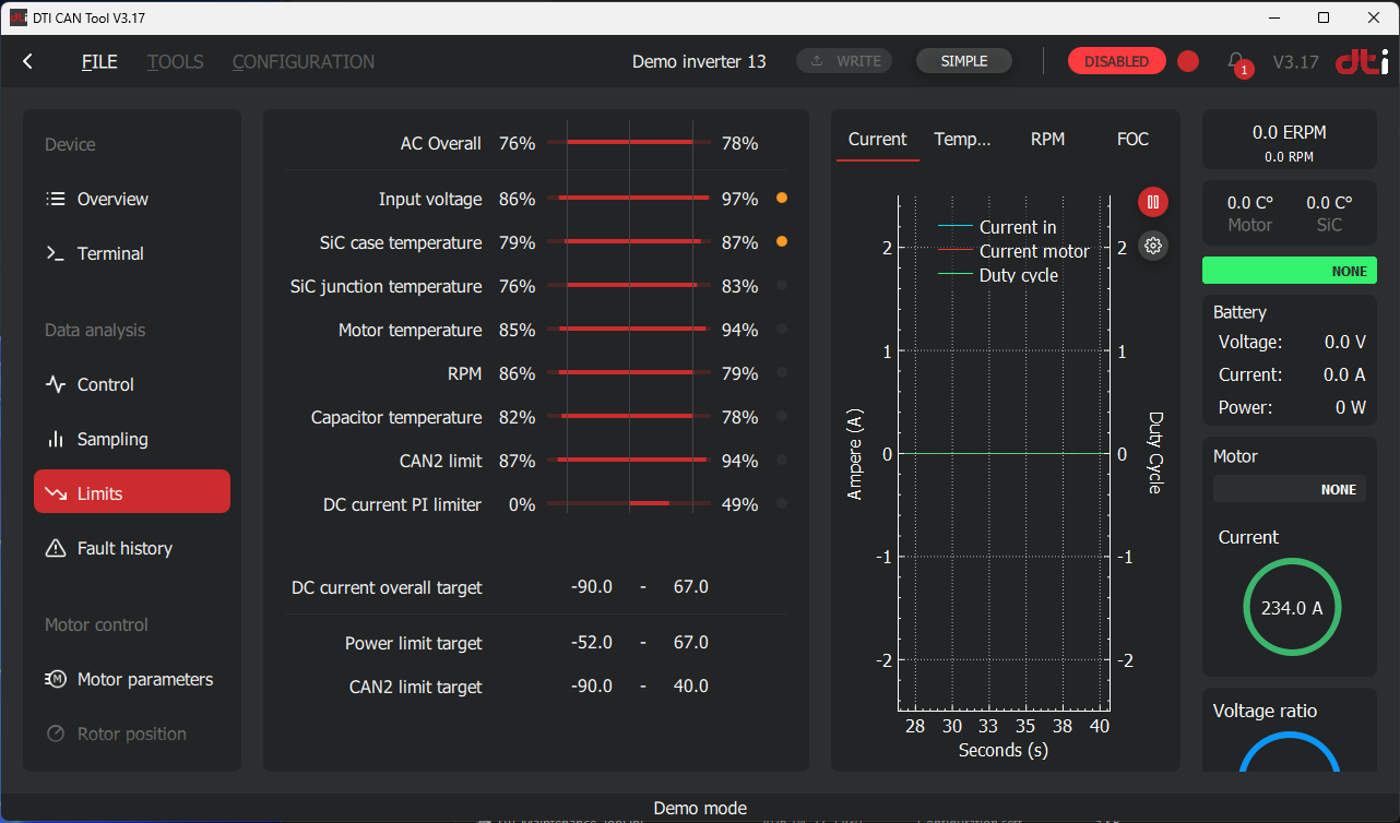
The tab is divided into two groups: AC limits are shown in the upper section and DC limits in the lower section. Each limit is displayed as a percentage:
- 0% — the limit is not active; no current reduction is applied
- 100% — the limit is fully active; the current output is suppressed to zero
Each limit entry also includes a status indicator: an orange dot is shown when the limit is currently active, and grey when it is not.
Torque estimation
The controller accepts a total AC peak phase current target (\(i_s\), in Apk) via the CAN2 interface. The decomposition into d- and q-axis components is handled internally by the MTPA and MFW algorithms — the user does not set \(i_d\) or \(i_q\) directly.
The electromagnetic torque of an IPMSM depends on both components:
where \(p\) is the pole pair number and \(\lambda_{pm}\) is the permanent magnet flux linkage.
Recommended method — Effective flux linkage with CAN2 feedback
A more accurate approach uses the actual \(i_d\) broadcast by the controller over CAN2 to compute an effective flux linkage at the current operating point:
The required q-axis current is then:
Because the commanded value is the total current magnitude \(i_s\), the d-axis contribution must be included:
The resulting \(i_s\) is the total AC current vector magnitude and can be sent directly as the current target via the CAN2 command interface.
This approach is exact within the accuracy of the motor parameters. It automatically accounts for the MTPA and MFW operating point at any load and speed, without requiring a fixed reference value or dynamometer characterisation.
For DTI F-MOT (\(p = 4\), \(\lambda_{pm} = 50.7\) mWb, \(L_d = 243\) µH, \(L_q = 371\) µH): all parameters are fixed — only \(i_{d,act}\) is read from the CAN2 broadcast at runtime.
Note
This method requires \(i_d\) to be available as a CAN2 broadcast message. Refer to the CAN2 Manual for the relevant message ID and scaling. When \(i_{d,act} \approx 0\) (MTPA disabled or near-zero load), the formula reduces to the simple proportional relation \(i_s \approx T\,/\,({\tfrac{3}{2}} \cdot p \cdot \lambda_{pm})\).
The accuracy of this method is affected by the broadcast rate of the CAN2 message carrying \(i_d\). A low update rate introduces lag between the actual and the read operating point, which can cause deviations in the computed \(i_s\) — particularly during transients. Configure the \(i_d\) broadcast period as short as the bus load allows to minimise this effect.
Validate the torque output
Regardless of the method used, it is recommended to validate the resulting torque output on a dynamometer before deploying the system in production. Several physical effects introduce deviations that cannot be fully compensated by calculation alone:
- Current-dependent inductance: \(L_d\) and \(L_q\) are not constant — they decrease with increasing current due to magnetic saturation. The motor parameters configured in the inverter are fixed values and do not capture this nonlinearity.
- Temperature-dependent flux linkage: \(\lambda_{pm}\) decreases as the permanent magnets heat up. The actual torque constant at operating temperature will differ from the value calculated using the nominal flux linkage.
- Other factors: manufacturing tolerances, rotor position sensor accuracy, and cross-saturation effects between the d- and q-axes all contribute additional error.
For applications requiring accurate torque control, characterisation on a dynamometer across the relevant current and temperature range is strongly recommended.